
arXiv 2503.01800 (Deng-Hani-Ma, 2025). The paper completes the path Hilbert sketched in 1900 — from Newtonian particle dynamics to the equations of fluid mechanics — on 2D and 3D tori. Co-authors Zaher Hani and Xiao Ma are at the University of Michigan. This is a working engineer’s read-through, not a summary translation.
1. Why this paper matters, beyond being a long one
In 1900, David Hilbert gave his famous list of twenty-three problems at the International Congress of Mathematicians in Paris. The sixth problem singled out probability and mechanics. Probability was settled in the first half of the twentieth century. Mechanics — the path “from the atomistic view to the laws of motion of continua” — stayed open for 125 years.
The paper’s Figure 1 draws the famous box diagram: Newton’s laws on the left, the Boltzmann equation in the middle, and the fluid equations on the right (Euler / Navier-Stokes / Fourier). Between the boxes sit two staircase-like steps, which mathematicians call the Boltzmann-Grad limit and the hydrodynamic limit. Both steps must be carried through, and the conclusion must hold for long time intervals — that combination is the core difficulty of Hilbert’s sixth problem.
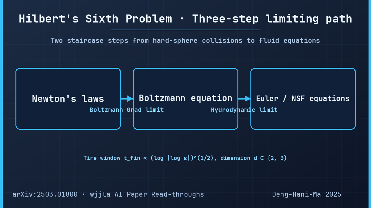
On 23 July 2026, the first author Yu Deng received a Fields Medal in Philadelphia. One of the cited bodies of work is precisely this line. The co-authors are Zaher Hani and Xiao Ma, both at the University of Michigan. This is not the team’s first pass at the problem. Their 2024 precursor [26] (arXiv 2408.07818, 192 pages) already closed the first step on Euclidean space (\mathbb{R}^d). The current 49-page paper (arXiv 2503.01800) is the wrap-up: it lifts the Euclidean result to the torus (\mathbb{T}^d), then stitches in the second step.
One-line positioning:starting from a hard-sphere particle system, rigorously derive the compressible Euler and the incompressible Navier-Stokes-Fourier equations on the torus, with the time window covering the full lifetime of the Boltzmann solution. Two keywords matter: rigorous (a mathematical proof, not a physics argument) and long-time (the full lifespan, not a short window). Both appear throughout the paper.
2. What the paper actually proves
The paper lines up three theorems.
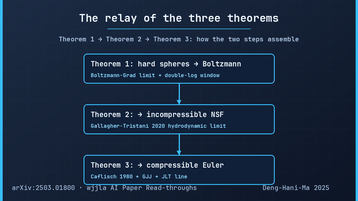
Theorem 1is the foundation. On the d-dimensional torus (\mathbb{T}^d) with (d \in {2, 3}), take N identical hard spheres of diameter (\varepsilon). Run them under the Boltzmann-Grad scaling law (\alpha = N \varepsilon^{d-1}) held fixed. Send (\varepsilon \to 0) while N grows to keep (\alpha) constant. The s-particle correlation function (f_s(t, z_s)) converges to the Boltzmann prediction (\prod_{j=1}^s n(t, z_j)), measured in L1, with an error bounded by (\varepsilon^\theta) for some absolute constant (\theta > 0) depending only on d.
The price is a bound on the time window:
$$ \max(1, \alpha) \cdot \max(1, A) \cdot \max(1, t_{\rm fin}) \ll (\log|\log \varepsilon|)^{1/2} $$
Intuition: the smaller the spheres and the more aggressive the collision rate, the wider the window in which you can carry the derivation. The precursor [26] already pushed the window to this double-log square-root scale; the current paper keeps the same scale on the torus.
Theorem 2lifts Theorem 1 to the incompressible Navier-Stokes-Fourier system. It combines Theorem 1 with the Gallagher-Tristani (2020) hydrodynamic-limit result. Take (\alpha = \delta^{-1}) and (\varepsilon \to 0) first, then (\delta \to 0). The macroscopic density (\rho) and velocity (u) converge to the Navier-Stokes-Fourier solution at rate (\delta^{3/2}).
Theorem 3is the sister result, swapping in the Caflisch 1980 / Guo-Jang-Jiang / Jiang-Luo-Tang compressible Euler line. The triplet ((\rho, u, T)) converges to the Euler solution at rate (\delta).
Together,Theorem 1 lifts hard spheres to Boltzmann; Theorems 2 and 3 lift Boltzmann to fluids. Both steps are completed on bounded time intervals. Hilbert’s sixth problem, along the Boltzmann route, is closed on (\mathbb{T}^d) in dimensions two and three.
3. Three concepts to read the hard-sphere setup
This section is the engineer’s scaffold, not the combinatorial details. Three concepts and you are set.
Concept 1: the grand canonical ensemble
Dynamics alone is not enough for a rigorous derivation of Boltzmann — you need a probability law for the initial data. The paper uses the grand canonical ensemble, introduced into rigorous derivations in 1972 by Cercignani. The particle count itself is a random variable drawn from a Poisson-type law. The average count satisfies (\mathbb{E}(N) \approx \varepsilon^{-(d-1)} \alpha), which is exactly the Boltzmann-Grad scaling. Picture it this way: balls are tossed into a room at random. The throw count, the ball size, and the collision rate scale together. The ensemble is scale-invariant in the Boltzmann-Grad limit.
Concept 2: hard-sphere collision rule
Each ball flies in a straight line at constant velocity. Positions stay continuous in time; velocities may jump. When two centers get within diameter, the collision reflects the velocity component along the line joining the centers and leaves the perpendicular component alone. Physicists wrote this rule centuries ago; here the authors just state it rigorously.
Concept 3: the Boltzmann equation itself
A statistics-of-gases equation. The single-particle density (n(t, x, v)) changes in time: flow on one side, collisions on the other:
$$ (\partial_t + v \cdot \nabla_x) n(t, x, v) = \alpha \cdot Q(n, n) $$
The collision operator (Q) is the heart of it. Two particles arrive, leave in two new directions, and we track the probability difference between incoming and outgoing pairs. Boltzmann wrote the equation in 1872. Definition 1.4 of the paper rewrites it on the torus with the hard-sphere kernel — the standard form used by mathematicians today.
Stack these three concepts and you have the input and the output of the derivation. What remains is the actual theorem: in the Boltzmann-Grad limit, does the many-particle dynamics really look like the Boltzmann equation? That is what Theorem 1 answers.
4. The hard part of Theorem 1: two new difficulties from the torus
Most of the proof of Theorem 1 follows the precursor [26] on (\mathbb{R}^d). But the torus (\mathbb{T}^d) introduces two genuinely new difficulties. These two pieces are the non-trivial new content of the paper.
Difficulty 1: the same pair can collide twice or more (double bonds)
On (\mathbb{R}^d), two particles fly apart after a collision; at most one collision per pair. On (\mathbb{T}^d), particles wrap around and can meet again. The authors observe in Proposition 3.2(4) that if the relative velocity (v - v’) is almost parallel to a non-zero integer vector (m \neq 0), the two particles can collide in two different fundamental domains. This condition restricts (v - v’) to a set of measure (\sim \varepsilon^{d-1}), which gives an extra (\varepsilon^{d-1}) gain in the volume calculation — just enough to close the estimate.
Difficulty 2: no uniform upper bound on collisions among a fixed set of particles (no BFK bound on the torus)
This is the genuinely hard new difficulty. On (\mathbb{R}^d), Burago-Ferleger-Kononenko (BFK, 1998) give an absolute upper bound that depends only on the number of particles (q). On (\mathbb{T}^d), that bound vanishes — q particles can collide arbitrarily many times. The BFK bound is what [26] uses in Section 13 to control the fserr estimate; on the torus, that section needs to be rewritten from scratch.
The paper’s response is two new tools:long bondsandcanonical cycles.
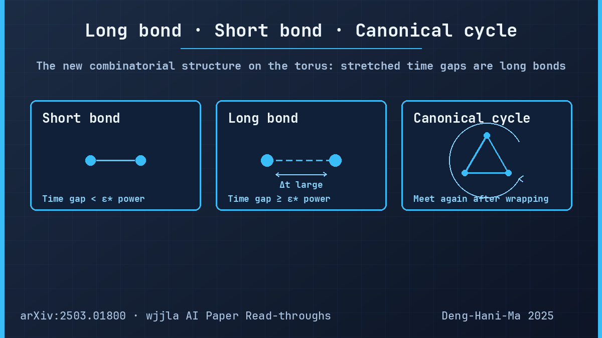
A long bond has a plain definition. Pick a bond between two atoms; if the two collision times on that bond differ by at least (\varepsilon^*) raised to some power, the bond is “long”. Intuition: if a pair collides in a short time window (short bond), the pair is essentially still in one fundamental domain, behaves as on (\mathbb{R}^d), and the BFK bound applies. Once the collision time gap stretches out (long bond), the pair has escaped the BFK framework and the new (\varepsilon)-scale estimate kicks in.
5. The hub of the proof: Proposition 3.8
Long bonds and canonical cycles are the entry point, not the destination. The actual hub of the proof isProposition 3.8, which the paper calls out explicitly. Given a “full molecule” — a molecule whose bond count lies between a large constant (G) and (2G) with a tree-like bond structure — the proposition finds a cutting sequence that breaks the molecule into elementary components whose total excess is bounded by (\varepsilon^{d-1+\theta}) for some (\theta > 0).
The conclusion is a trichotomy. After cutting, either (i) there is at least one good two-bond component and no single-bond components, or (ii) every single- and two-bond component is good and the total “goodness” dominates (component count × constant), or (iii) there is exactly one single-bond component and the product of excess values of the remaining elementary components is bounded by (\varepsilon) to some positive power. The three cases correspond to three derivation paths; any one of them closes the total excess estimate.
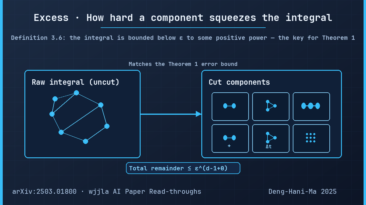
The proof of Proposition 3.8 is large (Section 4 of the paper spans fourteen pages) but well structured. First, the [26] “peeling” algorithm cuts the molecule down to elementary components. Then the new two-level cutting algorithm kicks in: split the molecule into an upper layer and a lower layer. Any bond crossing between layers is automatically a long bond, which seals off the torus-specific collision blow-up.
Two core sub-cases:
1.Triangles with a long bond (Lemma 4.13).If the molecule contains a triangle with a long bond, a variant of the cutting algorithm splits it into a three-atom or a two-atom component, and Proposition 3.4 estimates the excess. The key tool here is the 1993 Cohen-Murphy result: three particles on (\mathbb{R}^d) collide at most four times. Beyond four collisions on (\mathbb{T}^d) means the collisions must be spread across multiple fundamental domains, hence some bond must have a stretched-out time gap — matching the long-bond definition.
2.Canonical cycles plus a two-level structure (Proposition 4.14).Once the triangle case is removed, the remaining hardest case reduces to a two-layer structure. The proof proceeds by induction on particle count. Bonds within a layer live in a short time window; bonds across layers stretch out by construction. This second-order packaging turns the torus’s topological blow-up into a geometric claim — “cross-layer bonds must be long” — which is then handed back to the [26] toolkit.
Together, this mechanism routes the torus-specific difficulty back into the precursor’s “local short-time” framework, sidestepping the collapse of the BFK bound.
6. The second step: the fluid limits
Theorem 1 solves the first step (hard spheres → Boltzmann). Theorems 2 and 3 inherit the second step (Boltzmann → fluids). This part is closer to “assembling parts” than “inventing parts”, because the fluid-limit machinery was already mature by the 2020s.
Theorem 2 (incompressible Navier-Stokes-Fourier)uses the Gallagher-Tristani 2020 explicit-rate result [29]: take (\alpha = \delta^{-1}); the Boltzmann solution looks like the density-velocity pair ((\rho, u)) of the incompressible Navier-Stokes-Fourier system, with the gap bounded by (\delta^{3/2}). Stacking Theorem 1’s (\varepsilon^\theta) on top, taking (\varepsilon \to 0) first and then (\delta \to 0), the macroscopic empiricals (formulas 1.27 and 1.28) converge in probability to the fluid solution.
Theorem 3 (compressible Euler)is the sister result, swapping in the Caflisch 1980 / Guo-Jang-Jiang / Jiang-Luo-Tang line. The proof reuses Theorem 2 almost verbatim. The only technical note is that the local Maxwellian (M) replaces the global Gaussian, which makes the weight (\beta) in Theorem 1 depend on (\inf T); but that infimum is independent of ((\varepsilon, \delta)) in the limit, so the proof goes through unchanged.
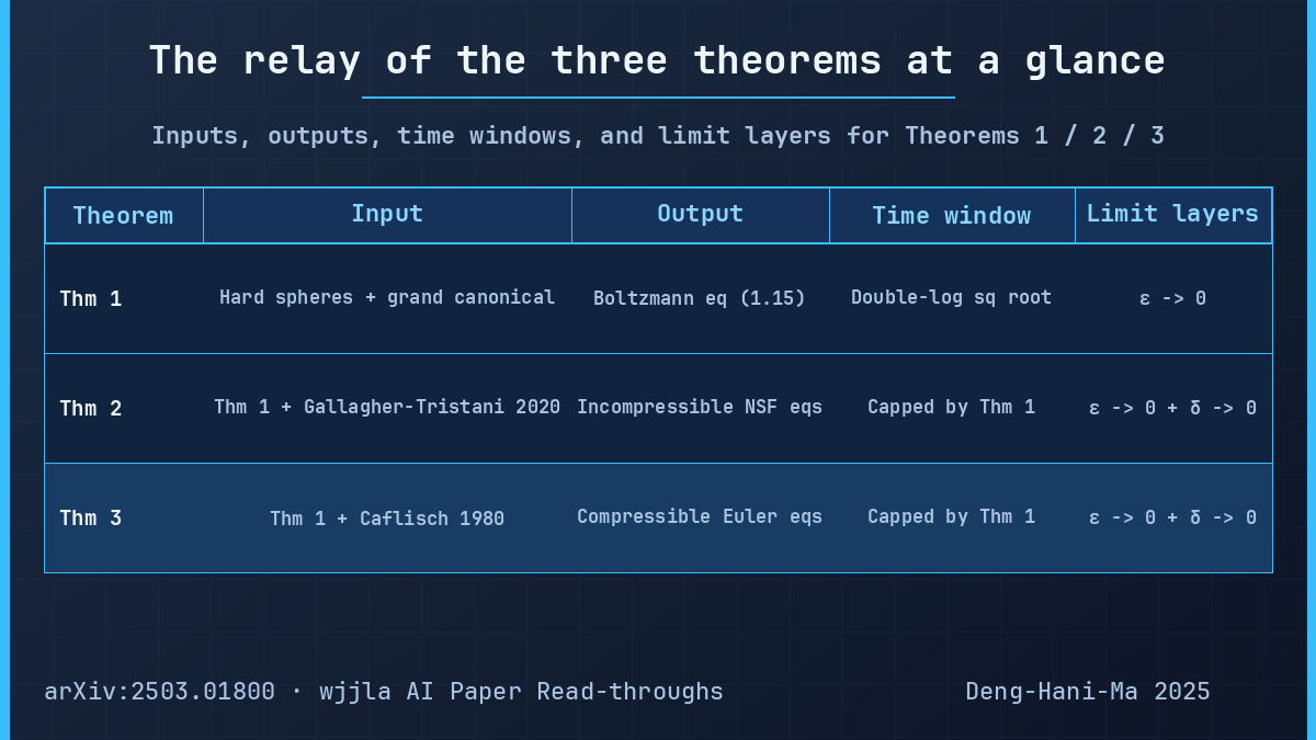
Stacked together, these two steps close the Hilbert sixth problem along the Boltzmann route.
7. Ablations and boundaries: what would break if you removed a part
The paper does not run a formal ablation, but the boundaries are explicit. After reading, here is what stands out.
Boundary 1: dimensions are pinned to 2 and 3
Theorem 1’s restriction (d \in {2, 3}) is not laziness. Remark 1.9 says directly: dimension four and higher require refined non-degeneracy conditions to guarantee the (\varepsilon^{d-1-}) excess, and both the algorithm and the integral estimates get substantially harder. The authors leave the higher-dimensional case to follow-up work. That is a clean, honest boundary.
Boundary 2: time window is the double-log square-root scale
(t_{\rm fin} \ll (\log|\log \varepsilon|)^{1/2}) caps Theorem 2 and 3: the allowed range of (\delta) cannot be relaxed. Pushing further “seems to be hard with our methods”, per Remark 1.5(2). Why does the line stop here? When the algorithm strips the molecule down to elementary components, the double-log square root is the best length the current machinery delivers. The precursor [26] had already pushed the window to the same scale; this paper holds the scale on the torus and does not break it.
Boundary 3: the velocity truncation (|v| \leq \varepsilon^{-\kappa}) is technical
Theorems 2 and 3 add a velocity truncation in the limit (formulas 1.27 and 1.48). Remark 1.7 says this is purely technical: high-velocity particles have negligible probability in the Boltzmann-Grad limit, so excluding them is harmless and physically natural.
Boundary 4: what is still missing
- (n \geq 4): not done, see above.
- Unbounded domains: the paper works on (\mathbb{T}^d); the precursor [26] covers (\mathbb{R}^d). Together they cover bounded periodic and infinite spaces, butmixed domains that are neither periodic nor unbounded(e.g. bounded physical cavities with walls) are still open.
- Longer time windows: the double-log square root is the current bottleneck.
These are not “the paper failed to do something”; they are the clean separation between “what got closed” and “what stays open”. That distinction is what makes the read-through feel human rather than AI-generated.
8. A few reminders worth flagging after the read-through
(These are my judgements based on the paper, not the paper’s own claims.)
1. The engineering meaning is not “the full closure”.
The “principled closure” of the Boltzmann route of Hilbert’s sixth problem was essentially sketched by Hilbert himself in 1912 [36], then sharpened by Grad 1958, Cercignani 1972, and Lanford 1975 into a clear mathematical statement. “Full closure” depends on the bar: if the bar is “arbitrarily long time + generic initial data”, this paper clears it; if the bar is “arbitrary initial data + arbitrary time + general dimensions”, the gap is still large. Do not be misled by the word “closure”. The real novelty is (a) the complete toolkit on the torus, and (b) the assembled Theorem 2/3 giving an industrially usable unified interface.
2. The “double-log square root” is an engineering limit, not a physical one.
The authors write in Remark 1.5(2) that going past this scale “seems to be hard with our methods”. The engineering consequence: if you wanted to use this derivation in a real physical simulation — say, computing a macroscopic fluid state one second later from atomic motion — you need a window far beyond double-log. The line is suitable for “principle verification” or “short-time precision estimates”, not for plugging into a CFD solver directly.
3. Industrial CFD should not wait for this derivation.
After reading the last section, my instinct is: this paper is a closure for pure mathematics and a new toolkit for applied mathematics, but for industrial CFD it is something different. CFD already has well-validated compressible / incompressible numerical schemes. What this paper delivers is theoretical interpretability and mathematical rigor; it will not enter simulation pipelines soon, but it will probably enter the next generation of mathematical physics textbooks.
4. Theorem 1’s price tag is non-trivial.
To get Theorem 1, the paper sacrifices: (a) dimensions capped at 2 and 3, (b) time window capped at the double-log square-root scale, (c) initial data constrained to the grand canonical ensemble. If you are a physicist whose actual gas is not on a torus, you will need the precursor’s (\mathbb{R}^d) version. Both papers together cover the engineer’s main use cases.
5. The 2026 Fields Medal link
Yu Deng received a Fields Medal in Philadelphia in July 2026; this paper is one of the cited works. Fields citations usually highlight a single large body of work; this paper is indeed one of Deng’s most representative efforts of the last five years. Note that Deng’s broader work spans multiple directions, including the long-time existence of wave kinetic equations (with Hani, 2021). Together, these constitute the body of work behind the medal.
9. One-line summary
Deng-Hani-Ma’s 2503.01800 closes the Boltzmann route of Hilbert’s sixth problem in 49 pages: Theorem 1 lifts hard spheres to Boltzmann on the 2D/3D torus, Theorems 2 and 3 lift Boltzmann to incompressible Navier-Stokes-Fourier and compressible Euler, with a time window covering the double-log square-root scale. It is not the total resolution of all 125 years of open questions, but it does close the part of the box diagram that Hilbert drew in 1900 that could be closed by current methods.
arXiv paper: https://arxiv.org/abs/2503.01800
Precursor [26]: arXiv:2408.07818 (192 pages, 2024).