Wang & Zahl, Volume estimates for unions of convex sets, and the Kakeya set conjecture in three dimensions, arXiv 2502.17655v1 (submitted 2025-02-26, 127 pages). One-line summary: the 3D Kakeya set has dimension 3, proved — and along the way, the 3D Tube Doubling conjecture and Keleti’s line-segment-extension conjecture both get closed as well. I read this paper all the way from the abstract through §12, and while I was at it I unpacked every bit of jargon that sounds like black magic.
1. Opening: two authors, and a problem that waited 108 years
The authors are Hong Wang and Joshua Zahl. Wang is a professor at NYU Courant and a permanent professor at IHES; she did her undergrad at Peking University (class of 2011) and her PhD at MIT under Larry Guth. Zahl is in the math department at UBC. Over the past three years these two have produced a trilogy that pushed a geometric problem from “almost there” to “fully proved” — it had been stuck for nearly a century. Wang just received the 2026 Fields Medal.
The story starts in 1917, in Japan. Sōichi Kakeya posed a question that sounds like something a grade-schooler could answer:if you rotate a unit needle (a unit-length line segment) on the plane, what is the smallest area the tip can sweep out?This later generalized into the Kakeya set: a compact set that contains a unit line segment inevery directionis called a Kakeya set. In 1971, Davies proved that in two dimensions, the Minkowski and Hausdorff dimensions of a Kakeya set are both 2 (full dimension). But in three dimensions and above, things were stuck — stuck for over half a century.
Picture it this way:a Kakeya set is like a parking lot where every direction of car is allowed to turn around— every direction has to have a “parking spot” big enough for one car, even if that spot is only a needle’s-width wide, but the directions have to cover a full 360°. In 2D you can easily imagine this lot being a normal disk; but the moment you lift to 3D, every direction needs a “solid-direction” needle that can be placed inside, and that’s counter-intuitively hard.
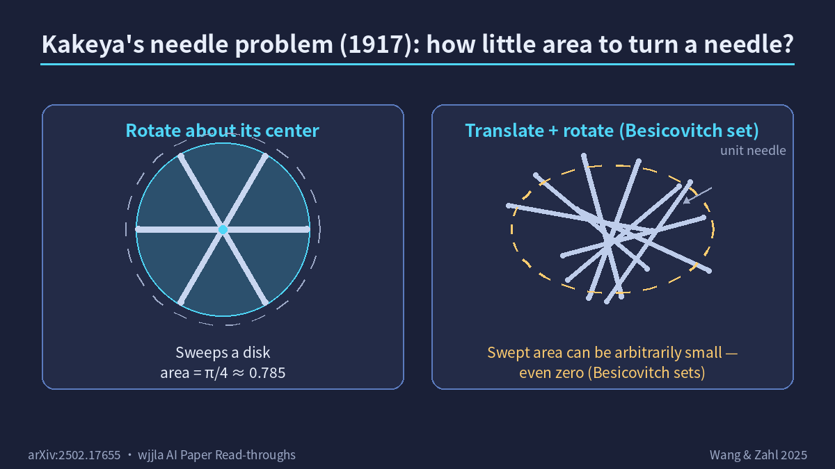
That picture is the original motivation for the problem: the area swept by one rotation, which intuitively looks like a circle but can actually be made into a “leaf shape” with smaller area — the cleverer you rotate, the closer the swept area gets to 0. Besicovitch gave constructions of this type with arbitrarily small — even zero — area (the paper mentions Besicovitch’s construction in R^2 in §1.6, see L664). But the dimension conjecture asks the converse: if a set “holds” needles in every direction, the dimension of that set must be 3.
Why is “dimension = 3” itself a non-trivial claim?Let’s pause here and pin down the word “dimension.”
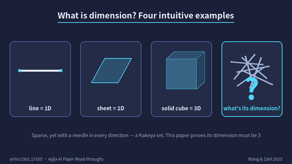
The most intuitive version: zoom a set in by a factor of ε and see how big it “looks.”Dimension doesn’t measure size, it measures “thickness”— how many independent directions the set “spans.” A thin line is one-dimensional (it only extends in one direction), a sheet of paper is two-dimensional (it spans two directions), a solid block is three-dimensional (all three directions are filled). When the Kakeya conjecture asks for “dimension = 3,” it means: the set that holds “every-direction” needles must spread out enough in all three independent directions — it cannot be squashed flat into a 2D sheet, squeezed into a 1D line, or collapsed into a pile of 0D points.
So “why can’t you cram different-direction needles into a 2D sheet” becomes the crux. It’s geometrically counter-intuitive, but for decades nobody in math could rule it out.
2. Why 3D was stuck for a century: laying out the half-century scoreboard
Partial results on the 3D Kakeya conjecture ran along two lines: a “hard bounds” line chasing dimension lower bounds, and a “soft tools” line building structural theorems.
Hard-bounds line:Wolff’s 1995 paper [27] (Rev. Mat. Iberoam. 11) proved that the Hausdorff dimension of a 3D Kakeya set is at least (n+2)/2 = 5/2. Later, Katz, Laba, and Tao ([16] in the paper) added a small positive constant c on top of that, reaching 5/2 + c. This line delivers “absolute lower bounds,” but numerically they’re still far from 3.
Soft-tools line:Starting around 2000, Bennett–Carbery–Tao’s multilinear Kakeya theorem ([1]) showed that any “counterexample” must be “planar” — needles stacked together must roughly lie near some plane. Guth ([9]) used his famous “grains decomposition” to show that any counterexample must be “grainy” — needles can be organized into rectangular particles. Butthe most critical link — stickiness — stayed stuck: you could say a counterexample is planar + grainy + sticky, and then what? That’s where it froze.
In 2014, Terence Tao laid out the Katz–Tao program in a lecture and blog post ([24]) as three steps: step 1, prove that any counterexample necessarily has planar / grainy / sticky structure; step 2, “multiscale” that structure, getting finer and finer descriptions; step 3, use Bourgain-style discretized sum-product tools to “falsify” that multiscale structure.
Wang and Zahl’s 2022 and 2024 papers [25][26] actually skipped step 1. They went straight to “assume the counterexample is sticky, derive a contradiction,” and “assume the counterexample has Assouad dimension <3, conclude it must be sticky.” But put together the two steps still leave a gap: Assouad dimension can be larger than Minkowski dimension, so [25][26] didn’t actually close the door on Minkowski dimension <3.
This 127-page paper is exactly the piece that fills that last gap. Instead of assuming the counterexample is sticky, it directly proves “if D(σ, ω) is tight, the counterexample must grow up to look sticky on its own,” then uses the sticky Kakeya theorem to derive a contradiction. Once this step closes, “3D Kakeya set dimension = 3” is fully proved.
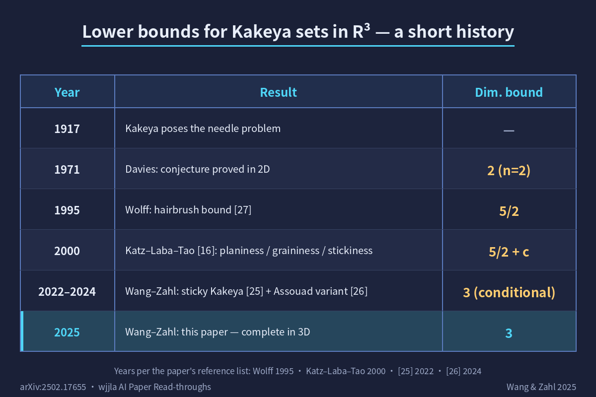
The concrete “old lower bound → new lower bound” jump: from Wolff’s 5/2 in 1995, through Katz–Laba–Tao’s 5/2 + c in the 2000s, all the way to 3. The roughly 30-year gap of the (5/2, 3) interval — from Wolff to this paper — got bridged in one go in early 2025.
3. The real main character of this paper is “volume estimates for unions of tubes” — Kakeya is just the corollary
This has to be said up front, otherwise you’ll drown in terminology reading the paper. The paper’s title is Volume estimates for unions of convex sets, and the Kakeya set conjecture in three dimensions. Kakeya is just the corollary. Theactual main theoremsare Theorem 1.2 and Theorem 1.9 (with Corollary 1.10 coming from the latter). What they say is:
Given a bunch of δ-tubes (needles of thickness δ and length 1), as long as they don’t “bunch up” inside any convex set (the technical name is Wolff axiom or non-clustering), the volume of the union of all those tubes is “almost” equal to the sum of the individual tube volumes — meaning the tubes spread outalmost disjointly, with no large overlap.
Aδ-tubeis a recurring core term. It’s just “a needle of length 1 and thickness δ pointing in some direction.” In a daily-life analogy, it’s adrinking straw— a straw has its own orientation (along its length), its own thickness (diameter δ), and its “volume” is δ² · 1 = δ² (cross-section area times length). When δ is small (a really thin straw), the volume δ² of one straw is very small; the volume of ten thousand thin straws added up is still only δ² · 10000, which doesn’t sound big — but what the paper proves is: when the straws satisfy the “no bunching up inside any convex set” condition, ten thousand thin straws can only occupy ~10000 · δ² of volume in total, no more than that; in other words, they really do spread out “almost disjointly,” with no significant overlap.
The nameWolff axiomcomes from Wolff’s 1995 paper [27], which introduced this kind of “non-concentration” condition: take any rectangular box (size a × b × 2) and wrap it around the tube family; the number of tubes that can fit inside can’t exceed the box’s cross-sectional area times 1/δ² by more than a constant factor. In other words, the tubes can’t “clump into a single bundle.”
Translated into everyday language, this is exactly"crowd control at the supermarket.“Imagine ten thousand straws drifting around a giant warehouse, each with its own orientation. The Wolff axiom says: in any a × b × 2 little box (cross-sectional area a × b), you can fitat most about a·b/δ² straws— the box’s cross-section sets the upper bound on how many straws it can hold, regardless of the straws’ directions. If you take a 1 × 1 × 2 little box and suddenly 100× more straws fit inside than its cross-section upper bound allows, that violates the Wolff axiom. The Wolff axiom is fundamentally a”spread-outness“hard constraint: straws can’t bunch up.
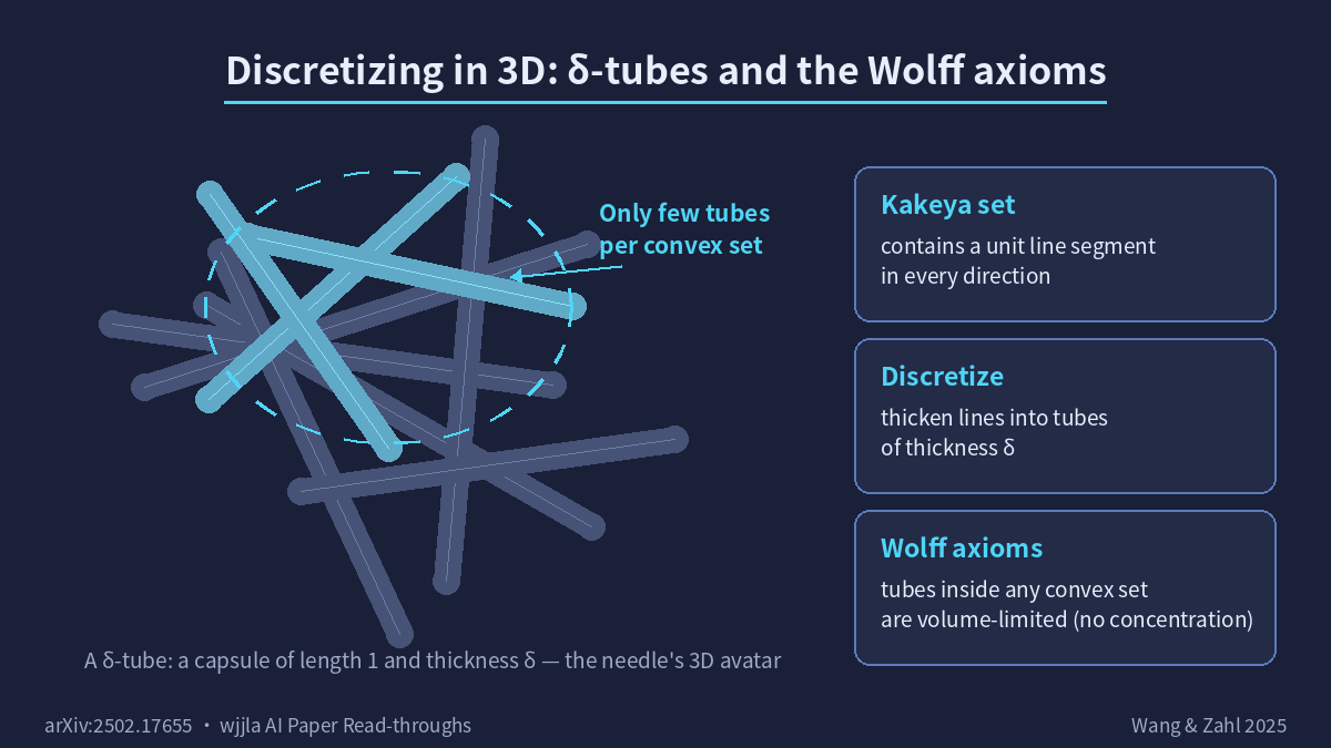
Intuitively: imagine you have tens of thousands of fine needles, one per direction. The Wolff axiom says “inside any a × b × 2 little box, these needles don’t suddenly bunch up 100×” — a hard constraint on “spread-outness.”
Kakeya sets satisfy this condition exactly: one needle per direction (δ-separated directions), so inside any a × b × 2 box in space, at most ~ab/δ² needles fit (the cross-section decides). SoTheorem 1.2 directly implies Theorem 1.1— that’s the “as a consequence” in the paper’s title, and where its real heft lives.
4. Core four-step argument: Wolff axiom → convex decomposition → two-scale grains → three moves → scale induction
The skeleton of the 127-page argument can be compressed into a 4-stage pipeline. I’ll cross-reference each stage with the paper’s own figure numbers.
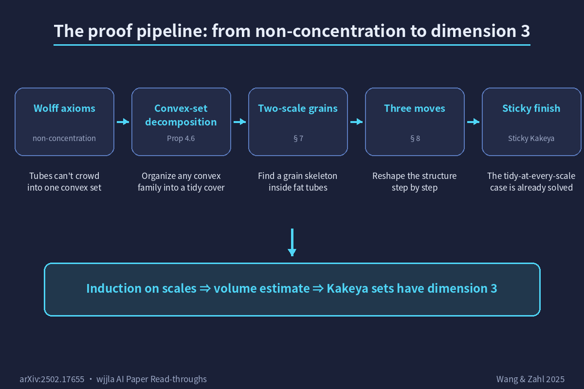
That figure lays out the four stages together: Wolff axiom constrains tube distribution → convex decomposition swaps the “tube family” for “wrapping convex sets” → two-scale grains packs tubes into rectangular particles → three moves nudges the particles “into place” → scale induction drives ω all the way down to 0.Memorize this five-part shape and the whole paper stops being a terminology jungle.
Step 1: Wolff axiom + convex decomposition(§4)
What’s happening here: first, swap the “tube family” for a more general vocabulary — any family of congruent convex sets.Why you have to do this:because working with δ-tubes directly is too specific; the geometry of how tubes interpenetrate each other is hard to describe. Once you switch to convex sets, you can organize the proof via nicer, more “linear” relations between convex sets: inclusion, covering, intersection.
Define two Wolff constants — the Katz–Tao Convex Wolff constant (CKT-CW, measuring “cannot bunch up inside any convex set W”) and the Frostman Slab Wolff constant (CF-SW, measuring “cannot bunch up inside slab slices”). The Frostman constant “inherits upward,” the Katz–Tao constant “inherits downward” — this dual pair is the engine behind every decomposition that follows. Proposition 4.6 is the key tool of this stage: given a family of convex sets, you can always find a family of “wrapping convex sets” W that control U from below via Frostman and from above via Katz–Tao, with errors absorbable into K.
One line on each symbol:CKT-CW is the normalized index of “how many tubes fit into a convex set W”— the smaller the value, the less the tubes bunch into W.CF-SW is the “thin-slice version” of the same idea, just that instead of any convex set W, it’s a slab of fixed thickness.Frostman inheriting upwardmeans spread-outness at a large scale can be transferred to finer sub-scales.Katz–Tao inheriting downwardis the opposite — spread-outness at a fine scale can constrain the coarse scale. These two “upward / downward inheritance” dual relations are like the two ends of a spring, and they’re the engine that makes every decomposition downstream actually work.
Step 2: Two-scale grains decomposition(§7)
What’s happening here: after Step 1 hands you a family of “wrapped convex sets,” take the tubes packed inside each convex set and run another round ofstructuring— organize them into rectangular “particles” (grains).Why you have to do this:because the relations between individual tubes are insanely complicated (each tube points in a different direction, tubes interpenetrate), but relations between rectangular particles are clean — just “fully contained / partially overlapped / disjoint” — and much easier to handle.
This is the second upgrade of Guth’s ([9]) grains idea. In [9], Guth proved that under “broad” assumptions, a tube family can be decomposed into δ × t × t rectangular particles (called grains), with t ≥ 1/√(#T). The paper turns this into atwo-scale version: first pick an intermediate scale ρ, and use ρ-tubes to wrap δ-tubes; inside each ρ-tube, run a grains decomposition independently, getting δ/ρ × c × c particles; rescale back, and you get a family of δ × ρc × c grains, called G. Two scales (δ and ρ) appear simultaneously — and that’s exactly the prerequisite for the “three moves.”
The wordgrainsin daily life is a row ofcandy skewers on a stick— a single bamboo skewer (the tube direction) threaded with chunks of similar-sized hawthorn berries (the particles), each chunk extending along the skewer’s direction.Why break tubes into candy skewers?Because skewers are easier to manage than a pile of loose hawthorn chunks: you can count how many skewers, how many chunks per skewer, how big each chunk is — and all those “sizes” and “counts” feed directly into a formula for estimating the volume.
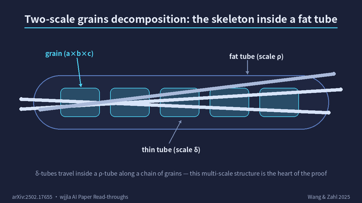
The c in the grain size isn’t arbitrary: c ≥ 1/√(#T[Tρ]) — grain size is inversely proportional to how many δ-tubes the ρ-tube contains; the sparser the packing, the longer the grains stretch. This formula (L950, §2.2) is the cornerstone of every subsequent magnitude estimate.What the two symbols mean in plain English:****#T is shorthand for “total number of tubes,” and Tρ is “the subset within some ρ-tube’s range” — together they say “the grain size at the current scale is constrained by how many thin tubes the parent thick tube at the previous scale held.”
Step 3: The three moves(§8)
What’s happening here: the grains coming out of Step 2 aren’t “in place” yet — some are too long, some too short, some too narrow.Why you have to do this:the scale induction downstream has strict requirements on grain “shape” (6 properties (i)–(vi)); without doing these three things, the induction’s input wouldn’t satisfy the conditions and the proof wouldn’t close.
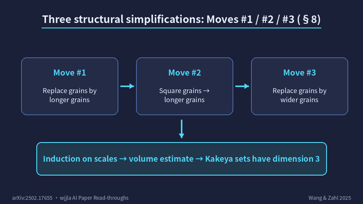
The authors do three things to push the grains “into place” — and put together, these three moves are likeorganizing a bookshelf in three motions: stand the leaning books upright (Move #1), stack books of different heights flush (Move #2), merge a few neighboring related books into one thicker volume (Move #3).
Specifically:
- Move #1(§8.1): swap the grains forlongergrains, ensuring c satisfies c ≥ δ^ζ · ρ·#Tρ / #T.What’s happening here:when the skewer chunks are “too small,” rebuild the skewer with chunks “big enough” to satisfy the grain-size lower bound.Why you’d throw the grains away and redo instead of patching:because every estimate downstream depends on this lower bound — if it fails, the formula blows up (diverges, useless). If the bound fails, just abandon this batch of grains and re-run the Guth decomposition from scratch — that’s an algorithmic “hard restart.”
- Move #2(§8.2): if the grains are “square-ish” (the b/c ratio in cross-section a × b × c is too large), use a Córdoba-style L² estimate to replace the grains withlongerones — stretched by a δ^(-ω/100) factor.What’s happening here:handle the case where “the grain’s cross-section is too square, not long enough along the skewer” — the candy chunks are too round, you need to stretch each chunk lengthwise.Why an L² estimate:because it pulls a “square-integrable” inequality tool into grain geometry — exactly what’s needed to push down the “cross-section / length” ratio.
- Move #3(§8.3): if CKT-CW gets too large, use an L² argument to expand each grain into a “hairbrush”: take the δ̃-neighborhood around it, swallow all the neighboring grains in, and end up with awidergrain.What’s happening here:when the “spread-outness” index at some scale has deteriorated (tubes start bunching up), merge nearby grains into one bigger “hairbrush” — a few small candy skewers combined into one big candy skewer.Why don’t you just delete the offending grains:because they carry real geometric information; deleting them throws away structure. You can merge, but not discard.
Each move either boosts c significantly or boosts ρ significantly — but both are capped at 1, so this iteration is guaranteed to stop after finitely many steps. That’s the classic “monotone and bounded, must converge” trick. When it stops, the grains satisfy all 6 properties (i)–(vi) (L948–970) — exactly the input for the induction on scale.
Step 4: Refined scale induction(§9 + §11)
What’s happening here: take Step 3’s “ideal grains” and run a more delicate induction — applying E(σ, ω) totwo layers, not just one.Why you have to do this:applying E(σ, ω) only once gives a volume estimate that’s not strong enough (it only knocks a little off ω, not enough to drive ω all the way to 0);using E on two layersstacks the estimate into “product form,” which is strictly stronger than using it once.
After Step 3 hands you “ideal grains,” the paper does something more delicate: it applies E(σ, ω) totwo layers— both on the δ-tubes inside each ρ-tube (fine scale), and on the ρ-tube family that each grain rescales to (coarse scale). Use E on both layers, and the resulting union-volume estimate comes out in a “two-layer product” form, which is strictly stronger than just using D(σ, ω) alone. This is the core of Proposition 1.7: it says each iteration knocks ω down by some g(σ, ω) > 0; with ω fixed, keep iterating and σ can be driven all the way down to 0.
The spirit of this induction is “climbing down stairs":each step of the staircase is a little lower than the previous one; as long as each step really does drop, even by a tiny amount (g(σ, ω) > 0), repeated walking gets you all the way down to the ground (σ = 0).Why does it have to be “two layers” instead of “one":a single-layer induction makes ω shrink too slowly, not enough iterations, so σ never reaches 0; stacking into product form makes the descent rate multiply out, and convergence becomes truly possible.What σ and ω mean roughly:σ is the “dimension deficit index” (closer to 0 means closer to full dimension); ω is the “spread-outness degradation index” (the larger it is, the more the tubes bunch up; the smaller it is, the more they spread out). The induction drives both parameters to (0, 0) at the same time.
Sticky Kakeya wrap-up(§10 + §2.4)
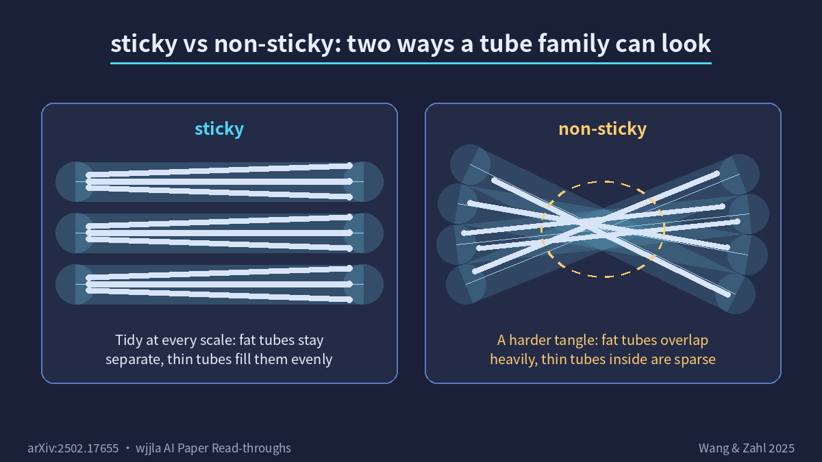
The killing blow: assume D(σ, ω) is tight (no slack) for some σ, ω > 0. Step 4 then forces T to be self-similar across multiple scales, satisfying the input of the Sticky Kakeya theorem. But [25] already proved that a sticky Kakeya set has dimension 3, which contradicts the tightness assumption on D(σ, ω). So σ and ω must both be 0 — meaning D(0, 0) and E(0, 0) both hold. That’s Theorem 1.9.
The wordstickyin everyday terms isa Russian nesting doll (matryoshka)— the outer doll wraps the inner, which wraps a smaller one, and so on; a sticky Kakeya set has exactly this structure: at every scale (zoomed out, zoomed in, zoomed in further), the set looks “like itself” — large-scale contains small-scale, small-scale contains even-smaller-scale, layer after layer of self-similarity.Why does this “nesting-doll” structure let a contradiction fall out:once you know a counterexample is sticky, [25] has already proved that a sticky Kakeya set must have dimension 3. But you also assumed the dimension is <3 (counterexample exists), so a counterexample can’t possibly be sticky — yet the previous step showed a counterexample must be sticky. Contradiction.
The tool used in this step is the Nikishin–Stein–Pisier factorization (§10.1, L5910): it fills out a sparse T (with tube count « δ^(-2)) up to δ^(-2) tubes, so that the Sticky Kakeya theorem can apply.The spirit of this toolis”a rubber band pulled as tight as it can go”— you have a bunch of tubes, but they’re too sparse (count « δ^(-2)), while the Sticky theorem needs δ^(-2) tubes to run. What Nikishin–Stein–Pisier does is “multiply” the sparse tubes up into a dense version — the equivalent of stretching a rubber band taut: a sparse set is rigidly expanded into a dense set, its “density” reaching the lower bound that the Sticky theorem requires.
5. Two bonus prizes: Tube Doubling and Keleti’s conjecture get closed in the same blow
Think it’s over? No — the paper also proves the 3D Tube Doubling conjecture (Theorem 1.12, L685) and Keleti’s line-segment-extension conjecture (Theorem 1.14, L698) as bonus.
Tube Doublingsays: thicken a bunch of δ-tubes by a factor of 2 (turn them into 2δ-tubes), and the volume of the thickened union exceeds the original union’s volume by at most a sub-polynomial factor δ^(-ε). The 2D version was already known (recorded in the paper’s §1.6); the 3D case had been stuck. Wang–Zahl’s Wolff axiom + convex decomposition package takes it down directly.
Keleti’s conjecturesays: if you have a bunch of line segments and extend each one into a full line, the dimension of the resulting line union equals the dimension of the original segment union. Keleti–Máthé ([23]) proved in 2022 that the n-dimensional Kakeya set conjecture implies the n-dimensional Keleti conjecture, so Wang–Zahl’s packagecomes with a free 3D Keleti conjecturethrown in.
Neither of these corollaries is “trivial to extract.” The paper gives a full proof of Tube Doubling in §12, using the same multiscale structural theorem from §11 together with the Nikishin–Stein–Pisier factorization.
6. The boundary: why doesn’t n ≥ 4 get closed at the same time?
The paper doesn’t spell this out explicitly, but I want to flag it after reading §1. There areat least three placesin the entire argument where the proof is specifically tied to three dimensions:
- TheWolff hairbrush boundin 3D gives an exponent of δ^(1/2) (around L240) — this is exactly what kicks off Proposition 1.8’s “D(1/2, 0) is true”; the entire iteration starts from this 3D-specific exponent.
- TheGuth grains decompositionis a 3D tool ([9], L487, §1.5); the paper does not discuss whether a high-dimensional analogue exists.
- Theσ ∈ [0, 2/3] range where Assertions D and E are equivalent(L302, Proposition 1.6) — the 2/3 comes from this paper’s 3D argument; how this range changes in higher dimensions, and whether the iteration still runs, the paper does not address.
So strictly speaking:n ≥ 4 remains an open problem.The paper’s methodology may provide a template for future work, but it does not directly transfer the result.
Keleti’s line-segment-extension conjecture (Theorem 1.14) and Tube Doubling (Theorem 1.12) are also closed only in 3D in this paper — these are 3D-specific byproducts, not simple n-dimensional generalizations of the Kakeya result.
7. Critical review: what’s good, what’s hard, and is it worth chewing through
What’s good:
- No tricks.The Katz–Tao program was proposed in 2014; it’s been 12 years now, and people kept trying to “sidestep the stickiness step” — every attempt failed. This paper just deals with stickiness head-on, leaning on the new observation “if D(σ, ω) is tight, the counterexample must be sticky on its own” (§2.4 summary) plus the Nikishin–Stein–Pisier factorization to fill out the sparse set. Reading the §2 proof sketch, the biggest feeling I had was: the “hooks” of this argument snap together extremely tightly — every step follows from the structure the previous step delivered, with no “inspired jumps.”
- The multiscale structural theorem(§7’s Proposition 7.5) is a standalone, reusable tool. Even if you don’t care about Kakeya, this “two-scale grains decomposition + 6 properties” framework is a piece of geometric measure theory you can cite again and again.
- Clear writing.For a 127-page paper, the first 22 pages lay out the whole skeleton — Definition 1.3 (non-concentration condition), Definition 1.5 (Assertions D/E), Theorem 1.2 + Theorem 1.9 + corollaries, all in §1; §2 gives the proof sketch. The detailed filling-in is §3–§12. This “conclusion first, proof second” style is necessary at 127 pages.
What’s hard:
- 3 Wolff constants + 5 moves/properties + 7 grain-dimension combinations— just memorizing the names takes a big table. The paper has a notation table in §3.2, but it’s easy to get lost on a first read.
- TheNikishin–Stein–Pisier factorization(§10.1) is new to most readers (including me) — at its core it’s a probabilistic argument that “uses random rigid transformations to fill out a sparse set,” requiring some probability + convex geometry background.
- 127 pages is not marketing.§6 (Assertions D and E equivalent) has a “4-way polychotomy” (L884–901, items (A)–(D)) that requires handling all four cases, each one chapter-sized on its own. This section is a grind to read.
Is it worth chewing through:
If you work in harmonic analysis / geometric measure theory / PDE, this is one of the most important papers of 2025 — absolutely worth chewing. My recommendation: start with §1 + the §2 proof sketch (only 22 pages), then decide whether to dive into the §4–§12 details.
If you work in a neighboring field (combinatorics, probability), at least read §1 + §1.4’s historical context + §1.6’s corollaries (14 pages total) — enough to build intuition for “what level of result is this.”
If you’re just a math enthusiast, I broke §2 down into the unpacking above — that’s basically the main storyline. Walk through it with the 8 figures and the core idea lands.
8. One-line summary
The 3D Kakeya set has dimension 3, and in early 2025 a 127-page paper closed this for good using the combo: Wolff axiom + convex decomposition + two-scale grains + three moves + Nikishin–Stein–Pisier factorization. A geometric problem born 108 years ago in Japan just got its period — drawn by a PKU class-of-2011 Chinese mathematician and her UBC collaborator. n ≥ 4 is still open, but the toolbox is built.
Figure placement index:
- fig01 (The Kakeya needle problem) appears in the upper half of Section 1
- fig06 (What is dimension, anyway?) appears in the lower half of Section 1, where the concept of “dimension” is introduced
- fig02 (Tubes and the non-concentration condition) appears at the end of Section 3
- fig05 (History of dimension lower bounds) appears at the end of Section 2
- fig07 (Proof pipeline at a glance) appears at the start of Section 4
- fig03 (Two-scale grains decomposition) appears at the end of Step 2 in Section 4
- fig04 (The three moves workflow) appears at the end of Step 3 in Section 4
- fig08 (Sticky vs. non-sticky) appears in the Sticky Kakeya wrap-up paragraph of Section 4